Technical Articles > Using Formulas in Table Cells
In some cases, it is necessary to use values from other table cells as an element of a formula or an argument of a function. Therefore, two kinds of cell reference types are provided that can be chosen by the FormulaReferenceStyle property to determine how references to table cells are specified: The R1C1 style and the A1 style.
R1C1 Cell Reference Style
R1C1 cell references are displayed using numerical row ('R' + number) and column ('C' + number) values. These values can be relative and absolute.
TX Text Control recommends to use the relative R1C1 style for cell reference operations. The notation of a relative R1C1 cell reference includes square brackets around the numbers. These numbers refer to cell positions relative to the table cell where the formula is defined.
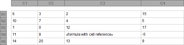
The following example illustrates relative R1C1 cell references in a formula that is defined at the fourth row (R4) of the third column (C3):
| Relative R1C1 Style Example | Description | |
| R[-3]C[-1] | Reference to table cell at first row (R1) and second column (C2) with value 3. | |
| R[1]C[-2] | Reference to table cell at fifth row (R5) and first column (C1) with value 14. | |
| R[0]C[1] | Reference to table cell at the same row (R4) and fourth column (C4) with value -5. | |
| R[-2]C[1] | Reference to table cell at second row (R2) and fourth column (C4) with value 5. |
An absolute R1C1 cell reference does not include square brackets around numbers. These values always refer to an absolute cell position, no matter in which table cell the formula is defined (e.g. R5C4 represents always the cell at the fifth row in the fourth column). This type of R1C1 references is supported, but should not be used, if the table is edited or the corresponding scope is pasted as a new table. In these cases, an absolute R1C1 cell reference returns invalid or incorrect values.
A1 Cell Reference Style
To refer to a specific table cell the A1 cell, reference style uses upper case letters (A-Z, AA-AZ, BA-BZ...) to define the cell's column (first column is A, second B etc.) followed by integers to specify the row (e.g. B3 refers to the table cell at the second column in the third row). This notation describes a relative cell reference and is the equivalent to the relative R1C1 cell reference style.
To apply absolute A1 cell references, the notation has to be extended with '$' signs to the left of the corresponding column or/and row to mark them as absolute. In this case, the cell reference does not depend on the table cell location where the formula is defined.
Cell Reference Ranges
Some functions accept argument lists where an unspecified number of values can be committed. If such values are stored in table cells, it could be very inconvenient to set these references one by one to the function. For those cases it is possible to apply cell reference ranges to define a matrix of table cells. Range definition is composed of two cell references, separated by a colon, where one reference represents the upper left and the other one the lower right of the scope to define.
The following example applies sample cell reference ranges to the SUM formula:
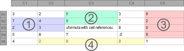
| Formula with Cell Reference Range | Description | |
| 1. SUM(R[-1]C[-2]:R[0]C[-1]) | Sums the values in the scope between R2C1 and R3C2 and returns 16. | |
| 2. SUM(R[-2]C[0]:R[-1]C[0]) | Sums the values in the scope between R1C3 and R2C3 and returns 14. | |
| 3. SUM(R[-2]C[2]:R[1]C[2]) | Sums the values in the scope between R1C5 and R4C5 and returns 20. | |
| 4. SUM(R[2]C[-1]:R[2]C[1]) | Sums the values in the scope between R5C2 and R5C4 and returns 19. |
LEFT, ABOVE and RIGHT
Another option to specify cell reference ranges is to use the LEFT, ABOVE or RIGHT flag. Each of these flags refer to the corresponding cell references next to the table cell where the formula is defined (e.g. SUM(ABOVE) sums the values of all cell references above the formula's table cell).
The following example applies the LEFT, ABOVE and RIGHT flags to the SUM formula:
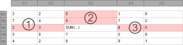
| Formula with Cell Reference Range | Description | |
| 1. SUM(LEFT) | Sums the values left to the formula's table cell and returns 5. | |
| 2. SUM(ABOVE) | Sums the values above the formula's table cell and returns 14. | |
| 3. SUM(RIGHT) | Sums the values right to the formula's table cell and returns 8. |